Introduction to Fourier analysis of time series
How to detect seasonality, forecast and fill gaps in time series using Fast Fourier Transform
In this article, I will show you the uses of the Fourier transform in time series analysis. We will use the Fast Fourier Transform algorithm, which is available in most statistical packages and libraries. Visualisations and code examples in Python supplements this article.
All are available in this notebook (Google Colab).
Although this topic often seems complicated, I will convince you that even basic use of Fourier analysis can give good results.
How to analyse weather data using Fourier analysis
Let’s assume that we work on some weather data.
| ds | temperature |
|---|---|
| 2008-01-01 | 0.49680824612499985 |
| 2008-01-02 | -2.8211083458333337 |
| 2008-01-03 | -5.7556919375 |
| 2008-01-04 | -7.374025225 |
| 2008-01-05 | -6.109025095833332 |
Full data: weather_sample.csv
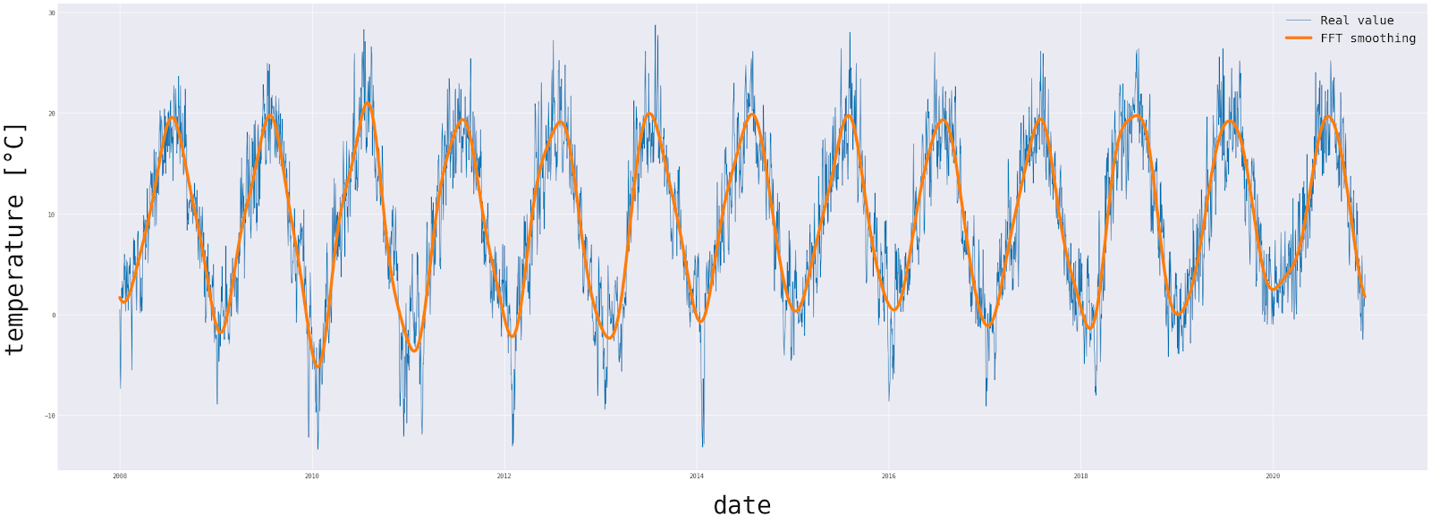
In our dataset is the average daily temperature for a certain location.
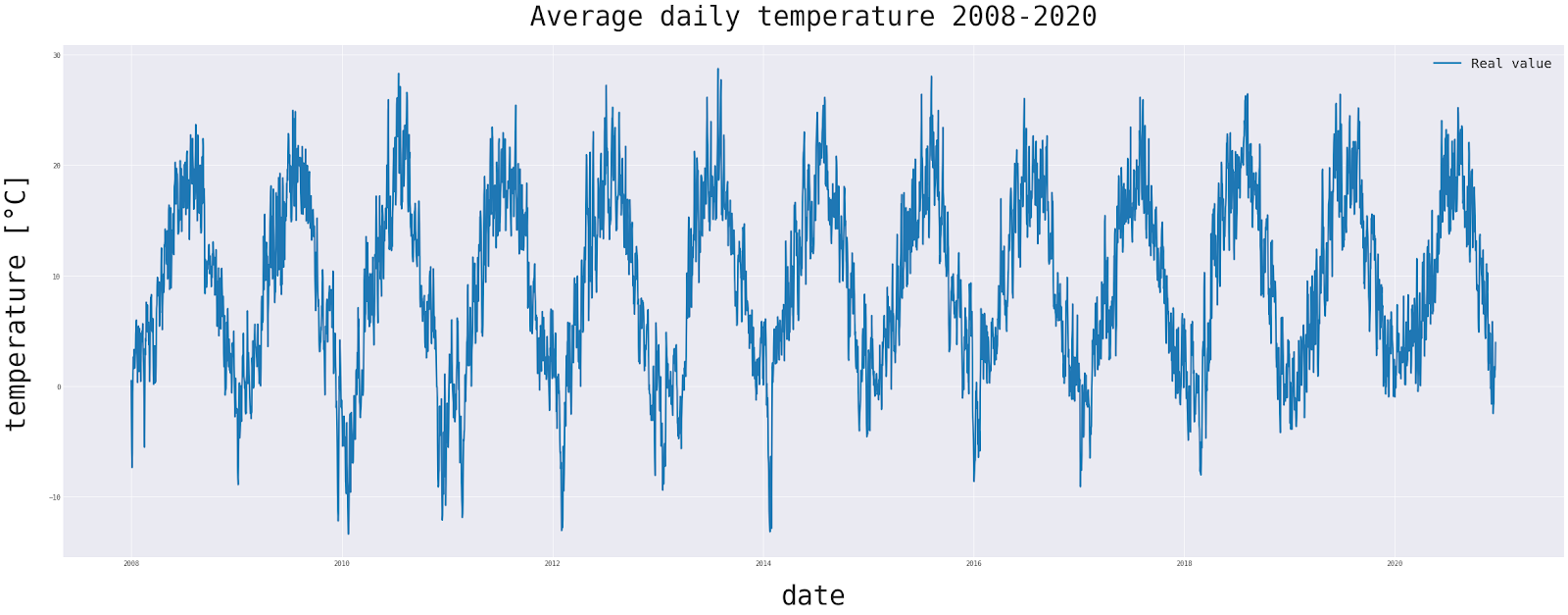
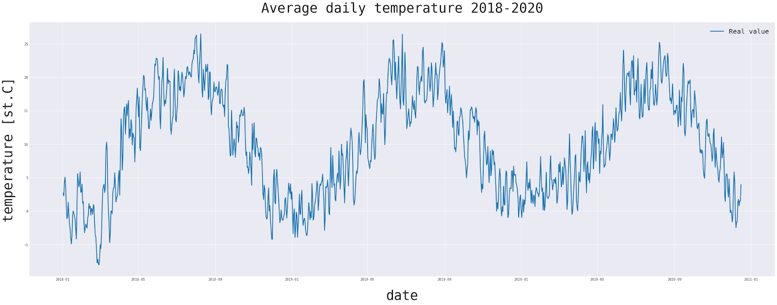
As we can see, a sinusoidal trend prevails throughout the year at a certain fixed frequency. If we can know what frequency this is, we can decompose the seasonality of this time series. This could be useful for improving forecasts or dealing with missing measurements.
Fourier analysis
Our goal is to take this single-variable periodic time series and decompose it into simpler periodic functions.
According to the theorem formulated by Joseph Fourier, any periodic function, no matter how trivial or complex, can be expressed as a composition (combination) of periodic components, known as the Fourier series.
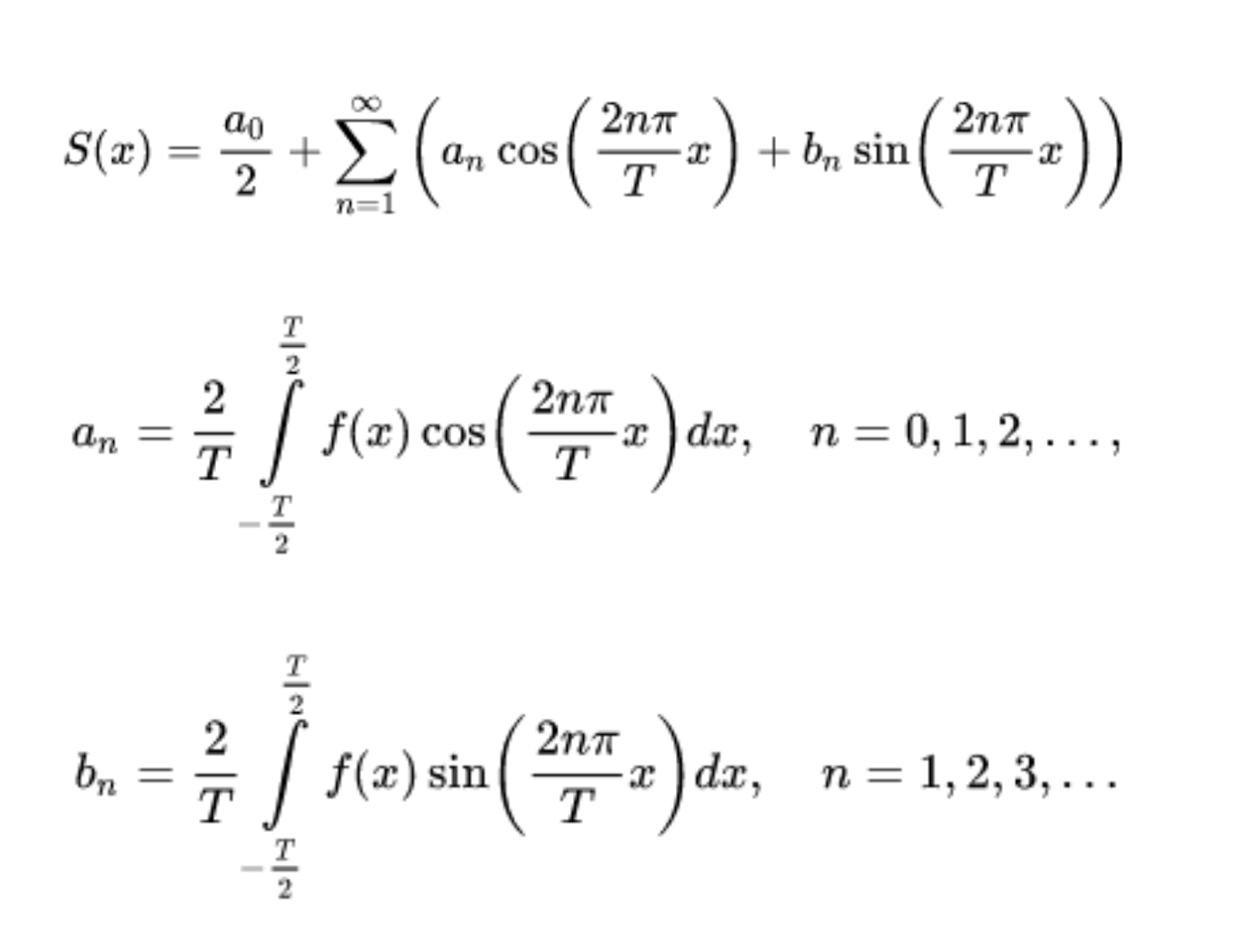
The method for expressing a function as a sum of sines and/or cosines, and for recovering the function from those components is called Fourier analysis. It does not matter if the function is non-sinusoidal. Any periodic time series is an infinite sum of sinusoidal components with coefficients.
Fourier analysis is the process of obtaining the spectrum of frequencies H(f) comprising a time-series h(t) and it is realized by the Fourier Transform (FT). Fourier analysis converts a time series from its original domain to a representation in the frequency domain and vice versa.
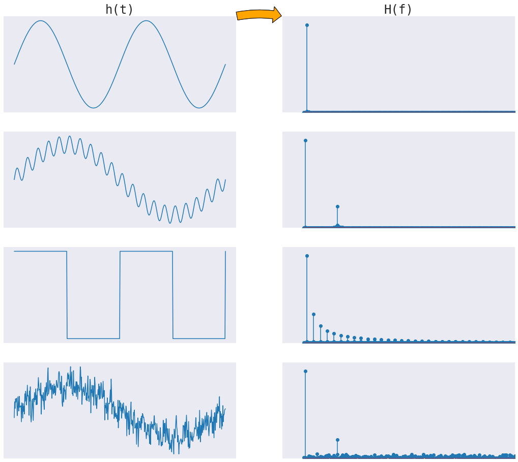
In simpler words, Fourier Transform measures every possible cycle in time-series and returns the overall “cycle recipe” (the amplitude, offset and rotation speed for every cycle that was found). Classical Fourier transform is for continuous functions. As our data is discrete, we will use a discrete counterpart of the Fourier transform.
We will apply the Fast Fourier Transform (FFT), an algorithm that computes the discrete Fourier transform (DFT) of a time series, or its inverse (IDFT). DFT has a great number of applications in physics, digital signal processing and compression, e.g. in MP3 and JPEG formats.
A good introduction to the FFT can be found in the NumPy library documentation:
How to detect time-series seasonality using Fast Fourier Transform
In the time-series data, seasonality is the presence of some certain regular intervals that predictably cycle on the specific time frame (i.e. weekly basis, monthly basis). Decomposing seasonal components from time-series data can improve forecasting accuracy.
There are many approaches to detect seasonality in time series, such as classical decomposition and seasonal extraction in ARIMA. We will use Fast Fourier Transform (FFT) to find the period of dominating seasonal components of time series. As an example, data that has one strong seasonal effect and residuals. Intuition suggests that temperature should have at least one year period. Let’s check it.
The procedure to extract seasonality from time-series is straightforward:
- Apply Fourier transform on the dataset to get frequency domain.
- Sort descending frequency domain by coefficients.
- Take the highest of these and get the periods by dividing 1 by the frequency.
nobs = len(data['temperature'])
temperature_ft = np.abs(rfft(data['temperature']))
temperature_freq = rfftfreq(nobs)

plt.figure(figsize=(10, 7))
plt.plot(temperature_freq[2:], temperature_ft[2: ])
annot_max(temperature_freq[2:], temperature_ft[2: ])

plt.xlabel('frequency (1/day)')
plt.show()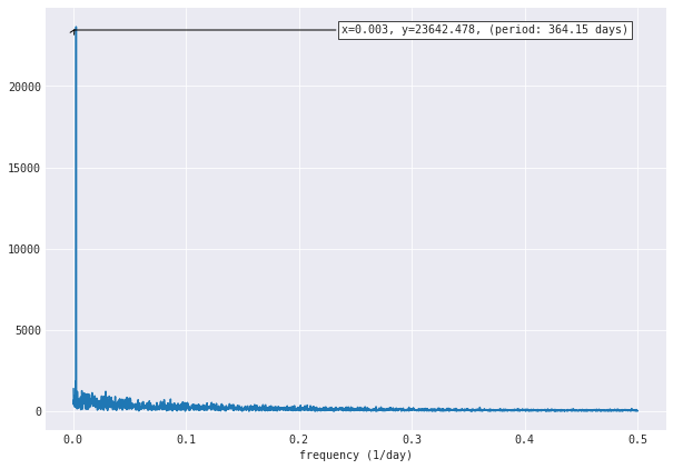
| freqency [1/day] | y | period [days] |
|---|---|---|
| 0.0027 | 23642.48 | 364.15 |
| 0.0023 | 1837.26 | 430.36 |
| 0.0025 | 1528.34 | 394.50 |
| 0.0004 | 1396.18 | 2367.00 |
| 0.002 | 1296.69 | 338.14 |
Full data: seasonality.csv
The result is quite predictable. Because of the seasons, the temperature fluctuates with the annual period. The result is consistent with this intuition.
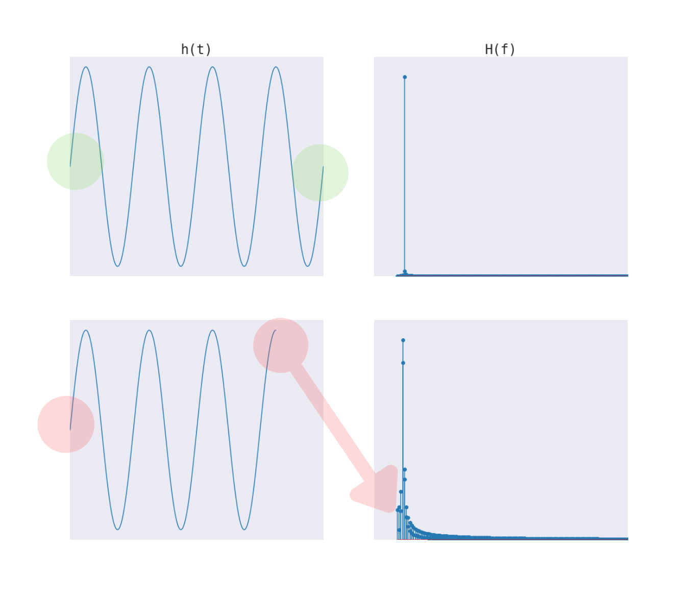
Sidenote: Spectral leakage
Because we have data from multiple full periods, we are unlikely to have to worry about spectral leakage. When we conduct FFT on a finite length time series, we assume the data repeats itself to infinity and connects the endpoint with the start point. But when there is a discontinuity, it spreads as a peak to the surrounding frequencies.
Here is an interesting article on how to deal with this problem:
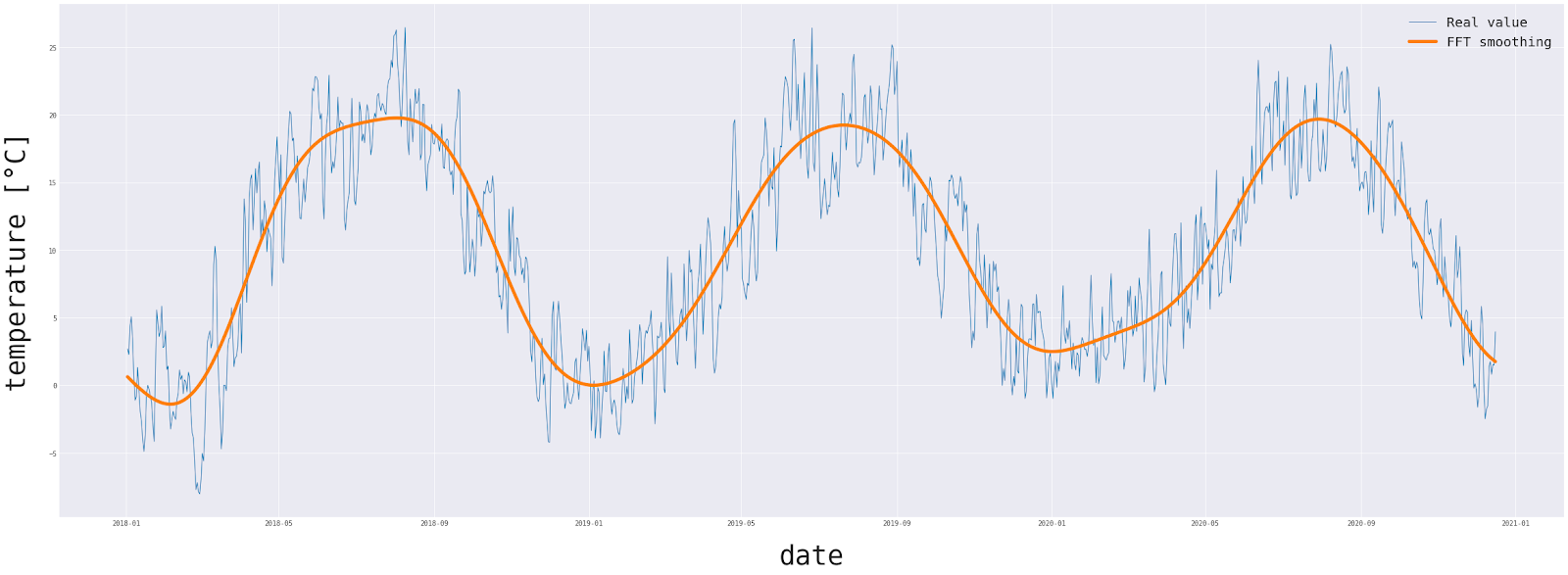
How to smooth time series using Inverse Fast Fourier Transform
Another use of FT is smoothing time series data. You can think about it as low-pass filtering that can be easily performed to remove components with a certain frequency and up, while information containing low-frequency components are retained. This can lead to the removal of unnecessary random fluctuations from the time series.
One might ask, why not use a moving average method or exponential smoothing. These methods do not exploit the observed periodicity in the data, So, for example, if there are gaps in the dataset, you can fill them with its estimations by adjusting the IFT parameters. This does not mean that we have to limit ourselves only to functions with noticeable seasonality.
Fluctuations of any function can be cut out to the desired frequency range. A similar approach can be used to get rid of seasonality in the data to increase the stationarity of the time series. In that case, a high-pass filter should be used.
The procedure is simple:
- Move to the frequency domain. (Fourier transform)
- Remove undesired frequencies.
- Move back to the time domain. (Inverse Fourier transform)
Let’s use this procedure.
Takeaways
As we can see Fourier analysis can help us capture the seasonality and can be used to decompose the time series data. Besides its usefulness, Fourier analysis is not a universal tool for all problems. FT is great for quickly creating predictive models for data with strong seasonality. Special events in your data, such as unexpected weather conditions, would not be predicted.
So, you can use Fourier Analysis whenever:
- You notice periodicity in data
- You need a quick forecasting model
- You want to fill gaps in the data
References
- Measuring Forecast Accuracy
- https://www.kaggle.com/residentmario/signal-decomposition-with-fast-fourier-transforms
- http://195.134.76.37/applets/AppletFourAnal/Appl_FourAnal2.html
- https://medium.com/towards-artificial-intelligence/seasonality-detection-with-fast-fourier-transform-fft-and-python-1021986d1e4f
- https://numpy.org/doc/stable/reference/routines.fft.html
- http://qingkaikong.blogspot.com/2017/01/signal-processing-finding-periodic.html