How to predict solar energy production
Efficient use of renewable energy sources with machine learning
Cite as: Rybnik, R. (2021). How to predict solar energy production: Efficient use of renewable energy sources with machine learning. Zenodo. https://doi.org/10.5281/zenodo.20562980
Code & data: solar-energy-forecasting-code-and-data.zip
Abstract
Solar photovoltaic (PV) energy production is highly dependent on weather, which makes its output difficult to predict. This article presents a practical, data-driven approach to forecasting the daily energy output of a rooftop PV installation in north-eastern Poland, using production data collected through the SolarEdge API together with historical weather data from Meteoblue and computed daylight information. Several forecasting methods are compared — naive and moving-average baselines and Facebook’s Prophet, with and without external weather regressors — and evaluated with standard forecast-accuracy statistics. The results show that adding a small number of readily available weather variables lets Prophet predict PV output with satisfactory accuracy and anticipate sudden changes in production.
Keywords: solar energy, PV forecasting, Prophet, time series, machine learning, weather data
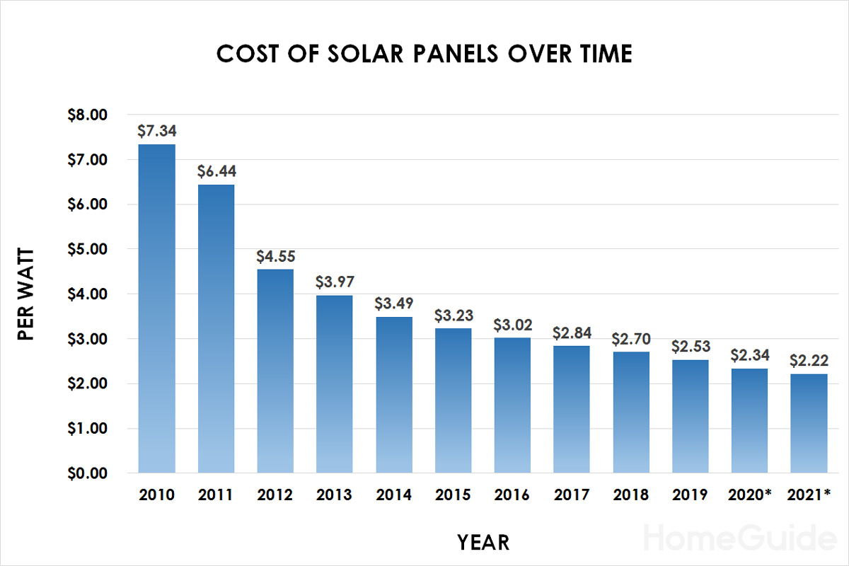
Solar power systems could be a key tool for energy production for the present and future generations. Solar energy is environmentally friendly and provides electricity to places where it is difficult to build conventional infrastructure. Photovoltaic (PV) cells become cheaper each year. Solar energy is cheaper than ever.
However, it has two huge obstacles: energy is produced only during the daytime and the amount of energy produced is highly dependent on the weather. Machine learning algorithms combined with weather data have the potential to overcome these barriers, which results with more efficient use of renewable energy sources.
In this article, you will learn about predicting time series depending on external (weather) conditions. I will show you how to improve your predictions using the domain knowledge of the target variable. We will go quickly through collecting data about energy production from the solar farm through its producers API. Next, we will analyze gathered data and select features for time-series forecasting. Finally, we will train and test several predictive models and identify the best, most suitable for the described case.
Why?
The problem with setting up solar power sources is that it is difficult to predict how much power it will generate once it’s built. Of course, we can quite accurately calculate the amount of solar energy reaching the Earth’s surface under ideal weather conditions. However, weather fluctuations and the unique microclimate of each location affect current energy production by renewable energy installations. This forces scheduling of tasks that require a lot of power.
To maximize the environmental and financial benefits of using renewable energy, we need to alter our habits. Making the electricity system intelligent and flexible will help optimize our behaviour and manage household energy consumption. Energy-consuming tasks can be scheduled for days or even hours of best weather conditions.
Lastly, knowing your system’s production tells you how quickly your solar system will return the investment.
Device
My friends have PV cells for more than a year.
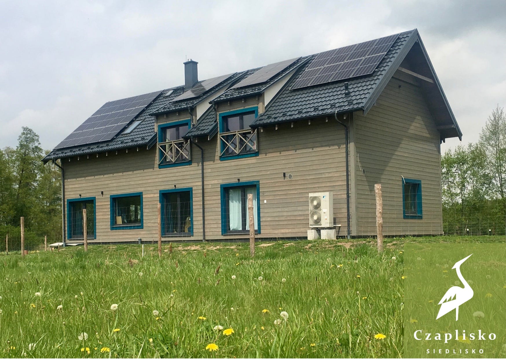
The whole installation has 31 panels that occupy 53 square metres of the roof. Inverter manages electricity generation. It is a device that converts direct current (produced by PV cells) into alternating current (used by household appliances), and manages the entire installation. Unused surplus is fed into the public electricity grid, which reduces the owner’s electricity bill.
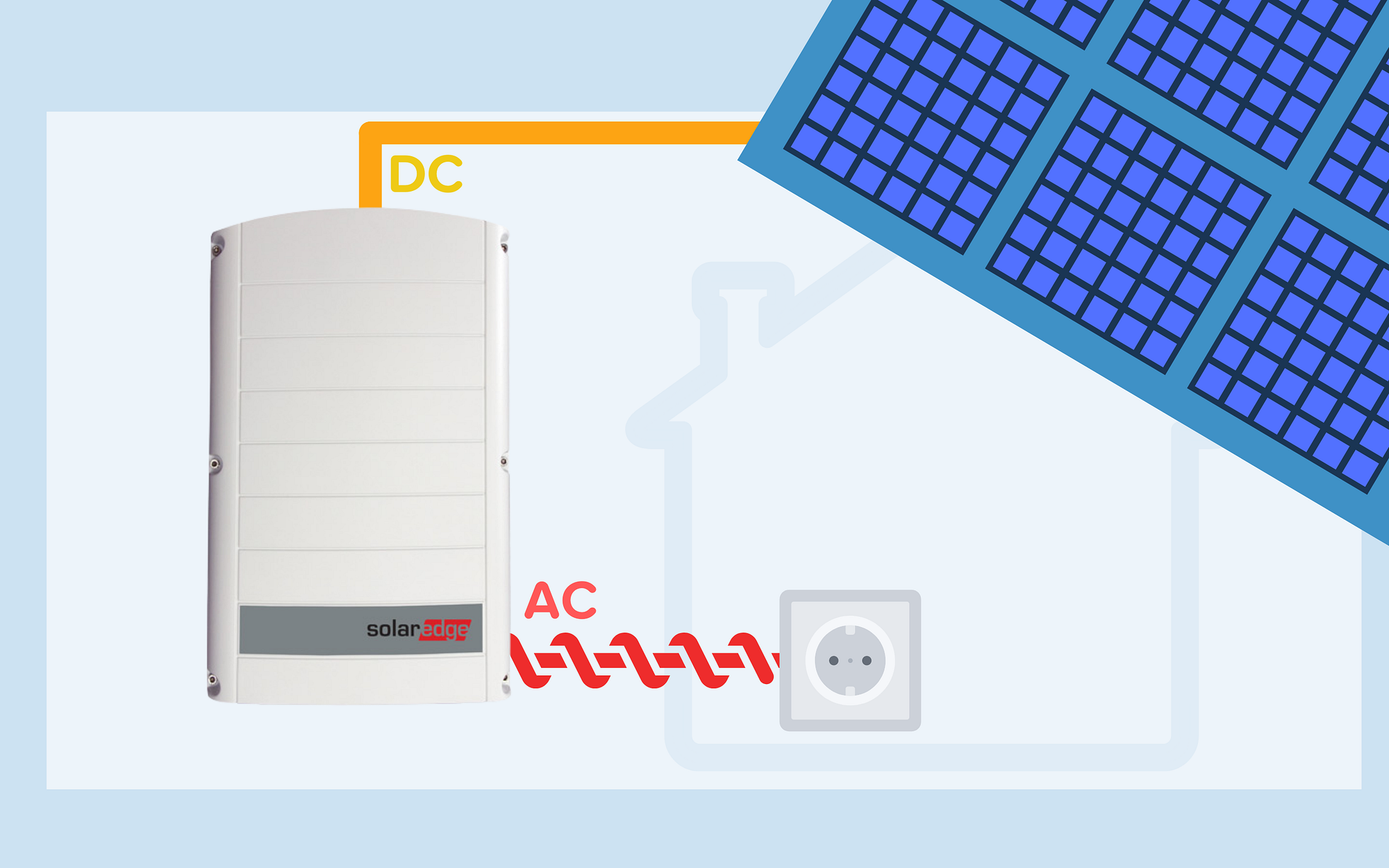
The inverter is manufactured by Solar Edge, which has equipped it with internet connectivity. The device sends statistics about energy production to the company, who makes it available to the owner of the installation via a mobile application, a website and API.
Acknowledgements
Special thanks are going to Czaplisko Siedlisko for sharing data from their solar farm.
Also, thanks Meteoblue for providing historical weather data for the location of the panels.
Data collecting
All code and data used in this article are available here: Solar Energy Forecasting in north-eastern Poland.
First, we need to collect and store data from SolarEdge API.
{
    "energy": {
        "timeUnit": "DAY",
        "unit": "Wh",
        "measuredBy": "INVERTER",
        "values": [
            {
                "date": "2020-12-09 00:00:00",
                "value": 2911.0
            }
        ]
    }
}
A typical response to an API request
To avoid repetition in the code, I sketched a simple API client.
class SolarEdgeClient:
    def __init__(self, key):
        self.key = key

    def show_key(self):
        print(self.key)

    def getDataPeriod(self, site_id):
        url = f"https://monitoringapi.solaredge.com/site/{site_id}/dataPeriod?api_key={self.key}"
        response = requests.request("GET", url, headers={}, data = {})
        data = response.json()
        return (data['dataPeriod']['startDate'], data['dataPeriod']['endDate'])

    def getSiteEnergy(self, site_id, start_date, end_date, time_unit='DAY'):
        url = f"https://monitoringapi.solaredge.com/site/{site_id}/energy?timeUnit={time_unit}&endDate={end_date}&startDate={start_date}&api_key={self.key}"
        response = requests.request("GET", url, headers={}, data = {})
        data = response.json()

        return data['energy']['values']

    def getSiteDetails(self, site_id):
        url = f"https://monitoringapi.solaredge.com/site/{site_id}/details?api_key={self.key}"
        response = requests.request("GET", url, headers={}, data = {})
        data = response.json()

        return data['details']


    def read_site_energy(self, site_id, start_date, end_date, time_unit='DAY'):
        site_details = self.getSiteDetails(site_id)
        datelist = pd.date_range(start_date, end=end_date).tolist()
        energyData = pd.DataFrame()
        for date in datelist:
            dailyData = self.getSiteEnergy(site_id=site_id, start_date=date.strftime("%Y-%m-%d"), end_date=date.strftime("%Y-%m-%d"), time_unit=time_unit)
            temporary_df = pd.DataFrame.from_records(dailyData)
            if(time_unit != 'DAY'):
                temporary_df['date'] = temporary_df['date'].apply(lambda date: Helpers.localtime_to_utc(date, site_details['location']['timeZone']))
            energyData = pd.concat([energyData, temporary_df])
        return energyData
It is worth noting that if you are dealing with time-series data, especially in hour or greater frequencies, you must take care of the time zones of all data sources. I recommend you convert datetimes to UTC timezone or to UNIX timestamps as soon as you import a timezone-aware dataset. For this purpose, I wrote some helper functions, which I have collected in one class as static functions. This makes the code more readable, without the risk of functions’ name conflict.
from astral.sun import sun
from astral.sun import daylight
from astral import LocationInfo
class Helpers:
@staticmethod
def localtime_to_utc(date, local_timezone="Europe/Warsaw"):
local = pytz.timezone(local_timezone)
naive = datetime.datetime.strptime (date, "%Y-%m-%d %H:%M:%S")
local_dt = local.localize(naive, is_dst=True)
utc_dt = local_dt.astimezone(pytz.utc)
return utc_dt.strftime ("%Y-%m-%d %H:%M:%S")
@staticmethod
def generate_daylight(start_date, end_date):
datelist = pd.date_range(start_date, end=end_date).tolist()
daylightData = pd.DataFrame(columns=['date','daylight','sunrise','sunset'])
for date in datelist:
daylight = Helpers.getDaylight(date)
daylightData = daylightData.append({
"date": date,
"daylight": daylight['duration'],
"sunrise": daylight['sunrise'],
"sunset": daylight['sunset']
}, ignore_index=True)
return daylightData
@staticmethod
def getDaylight(start_date, timezone="Europe/Warsaw"):
city = LocationInfo("Skitlawki", "Poland", timezone, LATITUDE, LONGITUDE)
s = sun(city.observer, date=start_date)
return {
"duration": (s['sunset'] - s['sunrise']).seconds,
"sunrise": s['sunrise'].strftime ("%Y-%m-%d %H:%M:%S"),
"sunset": s['sunset'].strftime ("%Y-%m-%d %H:%M:%S")
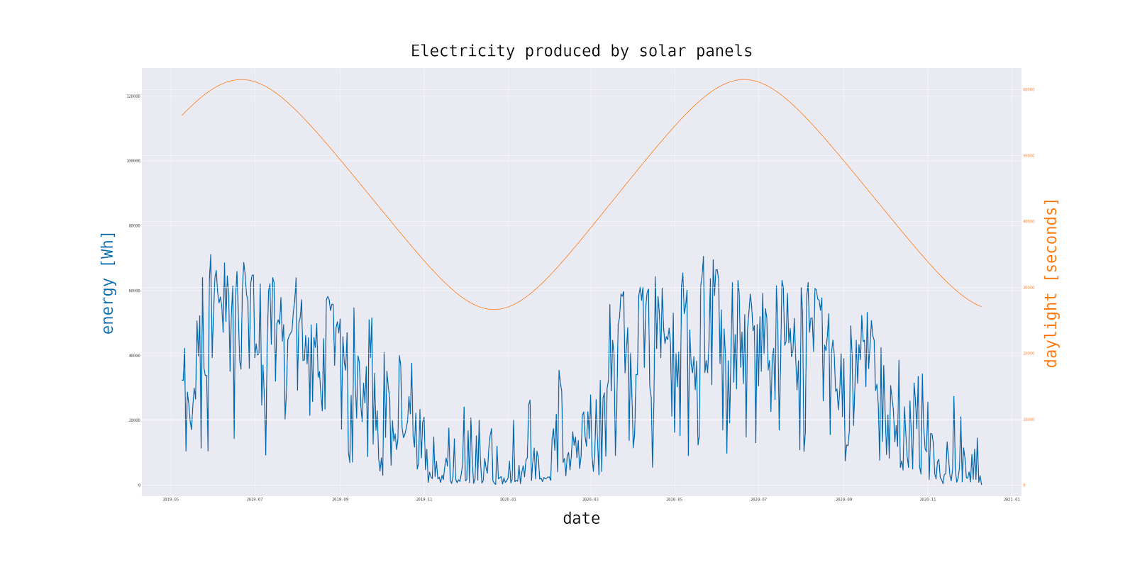
}We look at the data and establish success indicators
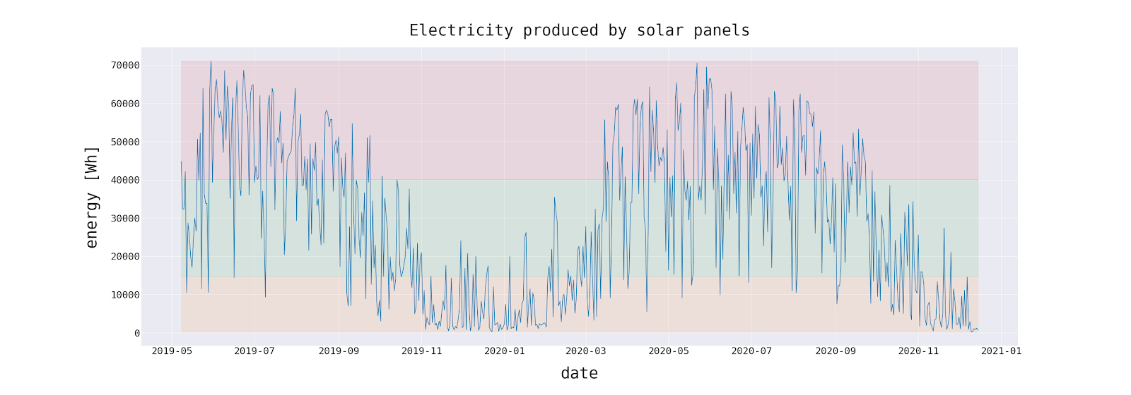
The first step to develop a predictive model for specific time series is to identify and understand the underlying pattern of the data over time. Data collected in the previous section contains the electricity output of the solar PV system, which is measured in kilowatt-hours (kWh). Just like in a smartphone’s battery, the kilowatt-hours unit describes how much energy is produced and can be used to power household appliances. 1 kilowatt-hour corresponds to the amount of energy consumed per hour by a 1,000-watt device.
| date | value |
|---|---|
| 2020-03-05 | 13895.0 |
| 2020-03-06 | 3245.0 |
| 2020-03-07 | 32336.0 |
| 2020-03-08 | 4228.0 |
| 2020-03-09 | 26802.0 |
| 2020-03-10 | 28464.0 |
| 2020-03-11 | 8922.0 |
| 2020-03-12 | 29895.0 |
Full data: energy_daily_sample.csv
Another metric is the current power production (measured in kilowatts), which describes how much power at the specific moment a solar panel can provide. For example, if the PV cells produce 1000 W at a specific moment, it is theoretically possible to supply two devices with the requirement of 450 W each and 100W remains. But to power, a 2500 W milling machine may require additional power to be obtained from the public grid.
After consulting the receivers of my forecasts, we have established that the information about the daily expected number of kilowatt-hours will be most valuable to them. The actual home equipment does not require sophisticated energy flow management techniques, so the moment the power of the system will not apply in the foreseeable future. In the following, we will therefore focus on the total energy produced (or to be produced) on a given day. The forecast horizon will be 5 days.
Simple forecasts
Before we will go deeper into forecasting based on external variables, let’s try to make a prediction having historical values of the target variable — daily electricity amounts produced by PV cells.
Naive forecast. This is a very basic method in which the predicted value is simply the value of the most recent observation. In our case, it will be energy produced the day before the prediction date.
Moving average. Another basic forecasting method is moving average. Moving average is rather a technical tool to analyse the time series, however, is extremely useful for forecasting long-term trends. In this case, we will use a simple moving average, which is a calculation that takes an arithmetic mean of a specific number of days in the past.
Code below tests those methods.
data = energy.copy()
data['cap'] = data['y'].max()
data['floor'] = 0.0
simple_methods = []
### Naive
MODEL = 'Naive'
data[MODEL] = data['y'].shift(periods=1)
arg = (data[MODEL], data['y'])
simple_methods.append([MODEL, *FES.all(*arg)])
### Moving Average
MODEL = 'Moving Average'
data[MODEL] = data['y'].rolling(4).mean().shift(periods=1)
arg = (data[MODEL], data['y'])
simple_methods.append([MODEL, *FES.all(*arg)])
simple_methods_df = pd.DataFrame(simple_methods, columns= ['Method', 'ME', 'MSE', 'RMSE', 'MAE', 'MPE', 'MAPE', 'U1', 'U2'])
display(simple_methods_df.set_index('Method'))
simple_methods_df.to_html('naive_and_moving_average.html', index=False)
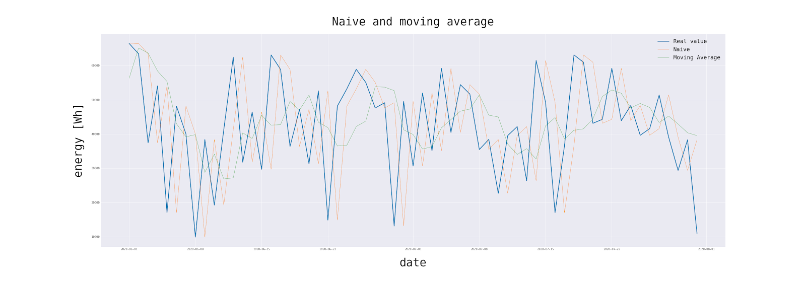
plot_data = data['2020-06':'2020-07']
fig = plt.figure(figsize=(40,14))
plt.xlabel('date',fontsize=40, labelpad=25)
plt.ylabel('energy [Wh]',fontsize=40, labelpad=25)
plt.plot(plot_data['y'], linewidth=2.5)
plt.plot(plot_data['Naive'], linewidth=0.75)
plt.plot(plot_data['Moving Average'], linewidth=0.75)
plt.legend(['Real value','Naive','Moving Average'], prop={'size': 20})
plt.title('Naive and moving average',fontsize=40, pad=30)
# plt.show()
plt.savefig('naive_and_moving_average.png')Note: We haven’t split the dataset for training and test sets yet. By definition of those methods, there is no risk of using data from the future.
How to evaluate forecasts (1)
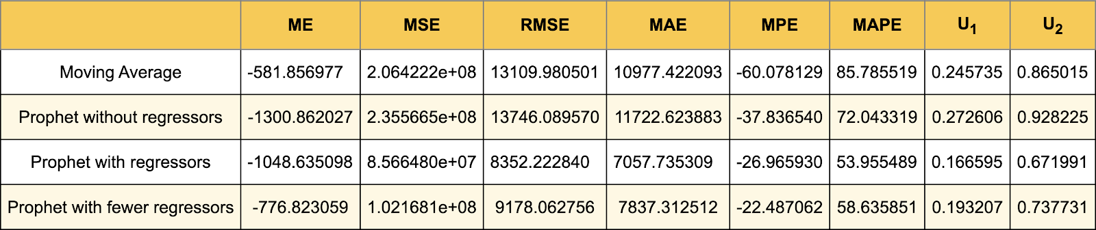
Now, for both methods, we should calculate several forecast evaluation statistics.
If you want to know more about forecast evaluation statistics, please read my article:
The table below shows the results of the evaluation:
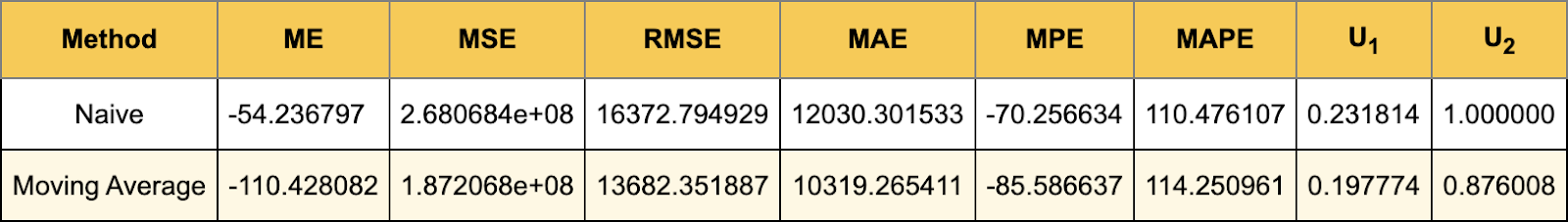
As expected, these methods are not very accurate. We will use those as a benchmark to evaluate more sophisticated ones. Because, if a more complicated model is less accurate than those forecasts, then there is something wrong. The main indicator of success is the ability of the model to inform about sudden changes in values of time series. No matter how well the trend fits the data, it can’t inform in time of sudden changes in production volume (because those are induced by external conditions).
In this context, to achieve our goal, we need a more advanced solution.
We need the Prophet
Our second shot will be Prophet library from Facebook. The Prophet is a procedure for forecasting time series data based on an additive model where non-linear trends are fit with yearly, weekly, and daily seasonality, plus holiday effects.
Creators of the Prophet advertise it as giving a reasonable forecast on messy data with no manual effort.
So, let’s test this declaration.
from fbprophet import Prophet
from fbprophet.plot import add_changepoints_to_plot
from fbprophet.diagnostics import cross_validation

# (...)

def prophet_without_regressors(train, test):
    m = Prophet(daily_seasonality=False, weekly_seasonality=False, yearly_seasonality=True, growth='logistic')
    m.fit(train)
    forecast = m.predict(test)
    forecast['yhat'] = forecast['yhat'].apply(lambda x: 0 if x<0 else x)
    return forecast.set_index('ds')['yhat']
How to evaluate forecast (2)
For the reliability of forecasts, the model can’t be trained using future data.

Therefore, for further evaluation and comparison of forecasts, we will use training and test sets. The size of the training set is typically about 20% of the total sample, depending on how large is the sample and the forecasting horizon. Since we have more than a year’s data and, also, the forecast is only to cover the next few days, we can use a more sophisticated method.
Instead of splitting the whole sample once, there are a series of training and test sets, separated from the sample as shown below.
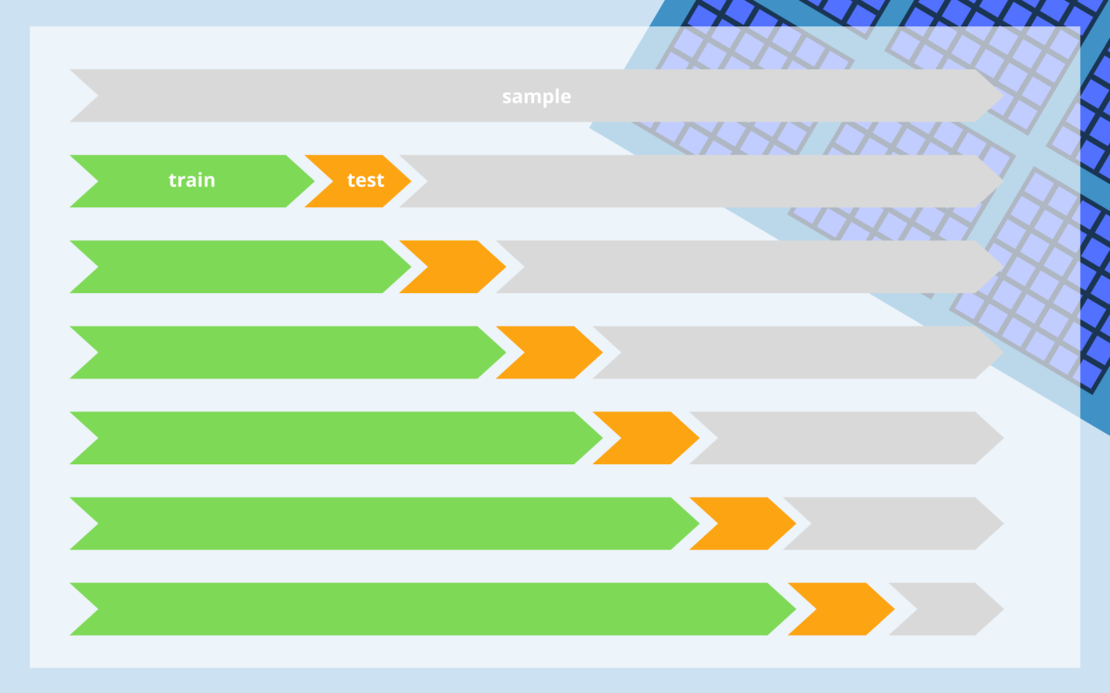
Each training set is used for the creation of a new model and then we calculate evaluation statistics using the corresponding test set.
def cross_validation(data, model=prophet_without_regressors):
    date_range = (data['ds'].min()+datetime.timedelta(days=365), data['ds'].max())
    datelist = pd.date_range(*date_range, freq='5D').tolist()
    evaluation_statistics = []
    for i in range(len(datelist)):
        if (i ** len(datelist) - 1):
            continue
        train_end = datelist[i]
        test_start = datelist[i] + datetime.timedelta(days=1)
        test_end = test_start + datetime.timedelta(days=5)
        if(test_end > data['ds'].max()):
            test_end = data['ds'].max()
        else:
            test_end = datelist[i] + datetime.timedelta(days=5)
        train_end = datetime.datetime.strftime(train_end, '%Y-%m-%d')
        test_start = datetime.datetime.strftime(test_start, '%Y-%m-%d')
        test_end = datetime.datetime.strftime(test_end, '%Y-%m-%d')

        train = data[:train_end].copy()
        test = data[test_start:test_end].copy()
        train['ds'] = train.index
        test['ds'] = test.index

        evaluation_statistics.append([f":{train_end} | {test_start} - {test_end}",*FES.all(model(train, test), test['y'])])
    evaluation_statistics = pd.DataFrame(evaluation_statistics, columns= ['period','ME', 'MSE', 'RMSE', 'MAE', 'MPE', 'MAPE', 'U1', 'U2'])
    return evaluation_statistics
It reproduces the real way of evaluating the forecast, as forecasts will be converted once every 5 days.
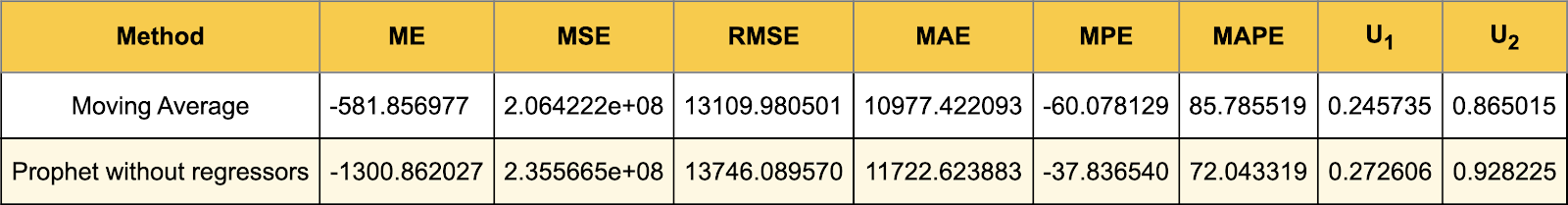
The Prophet is not doing better than the moving average. By the nature of the problem, it cannot take full advantage of the possibility of matching seasonality (after all, sunlight does not show weekly or monthly seasonality). MAPE for Prophet is slightly lower than for moving average. This suggests that it reacts to trend changes a little faster. Another statistic — Theil’s U₂ is less than 1, so both models are doing better than naive.
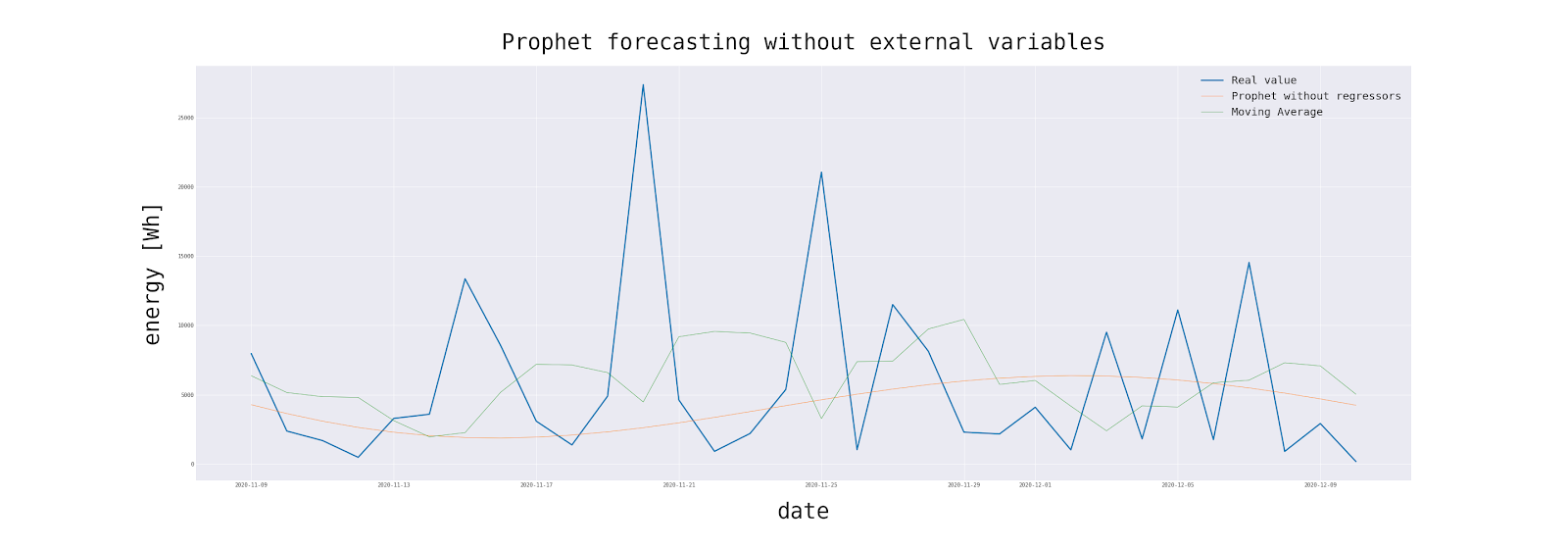
However, after a visual inspection of the chart of Prophet’s forecasts, it is encouraging to add external variables.
What are the factors that affect solar panels’ efficiency?
Theory
The kilowatt-hour production of a solar system depends on how much sunlight hits the panels and for how long. (source)
The amount of available sunlight depends on the local solar resource, weather conditions, panel orientation, amount of shading, system design and type of mounting (ground or roof mount).
Every installation is different. Things like the angle of PV, wiring and location-specific weather conditions could lead to short-term variability in results.
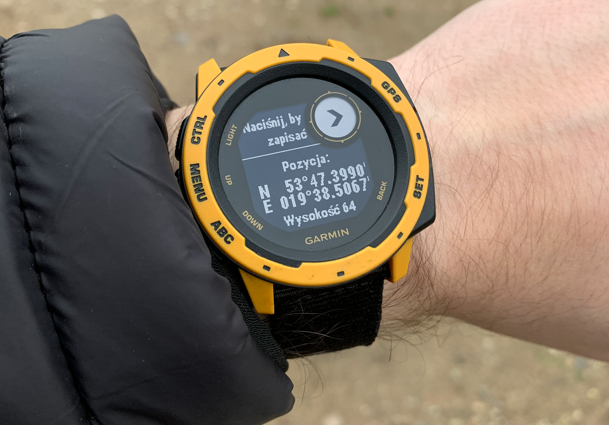
Location
Different parts of Earth’s surface receive different amounts of sunlight.
Weather conditions
Variables that may have a physical impact on the production of electricity by PV cells:
- air temperature,
- precipitation,
- snowfall,
- relative humidity,
- cloud cover,
- sunshine duration,
- solar radiation.
Cloud coverage does not mean that no sunlight will reach solar panels, but the amount will be reduced. Moreover, PV cells are often installed on the roofs of high buildings. Because of the lack of availability of reliable forecasts for every variable, not all of them will be used in the final model.
The approach proposed in this article is customizable for all installations and is independent of any device-specific characteristics (such as declared efficiency of PV cells). Also, the side goal is to use regressors easily accessible in most weather forecast services.
Temperature
Interestingly, air temperature is important not because it correlates with sun activity only. The efficiency of the PV cell depends on its temperature, which increases when the temperature drops and decreases when the temperature rises.
Weather dataset
As you know from previous sections, reliable weather data is crucial to the short- and long-term prediction of energy production. We should distinguish between two types of weather data: historical (from real-world measurements) and forecasted.
Just like in our future solar energy model, the weather forecast is also modelled. When creating models you should always focus on the domain of the problem and decide whether the model should be trained using historical weather forecasts or rather using past real measurements.
For example, if you have to predict the purchase of tickets to an amusement park, you better take into account the weather forecast, because consumers often consider it when they are planning such activities. The advantage of this approach is also that (assuming the stability of the weather forecast error itself) the weather forecast error will have an easier predictable impact on the final predictions.
On the other hand, if you are to predict the results of physical quantity measurements, it will be better to take into account real measurements of past predictors. Then the resultant forecast error will have a more difficult to analyse random distribution (resulting from interferences between the resultant model and weather forecast model). But, at the same time, the model will be resistant to changes in weather modelling.
In the solution described in this article, I used historical data for the weather, because available sunlight is variable depending on real physical conditions. Unfortunately, there are no weather stations near the location of the solar panels. But simulation data could be a good compromise.
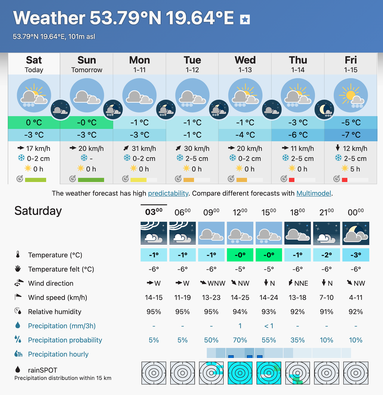
Meteoblue
Courtesy of Meteoblue, I was given access to historical weather data for the location of the solar panels. Their product history+ offers consistent weather simulation data in hourly resolution since 1985. Higher-resolution data are available since 2008 for nearly every place on Earth. Meteoblue history+ is a paid service, but you can test it for free with full historical data for Basel, Switzerland. For other locations, data is limited to the last 2 weeks.
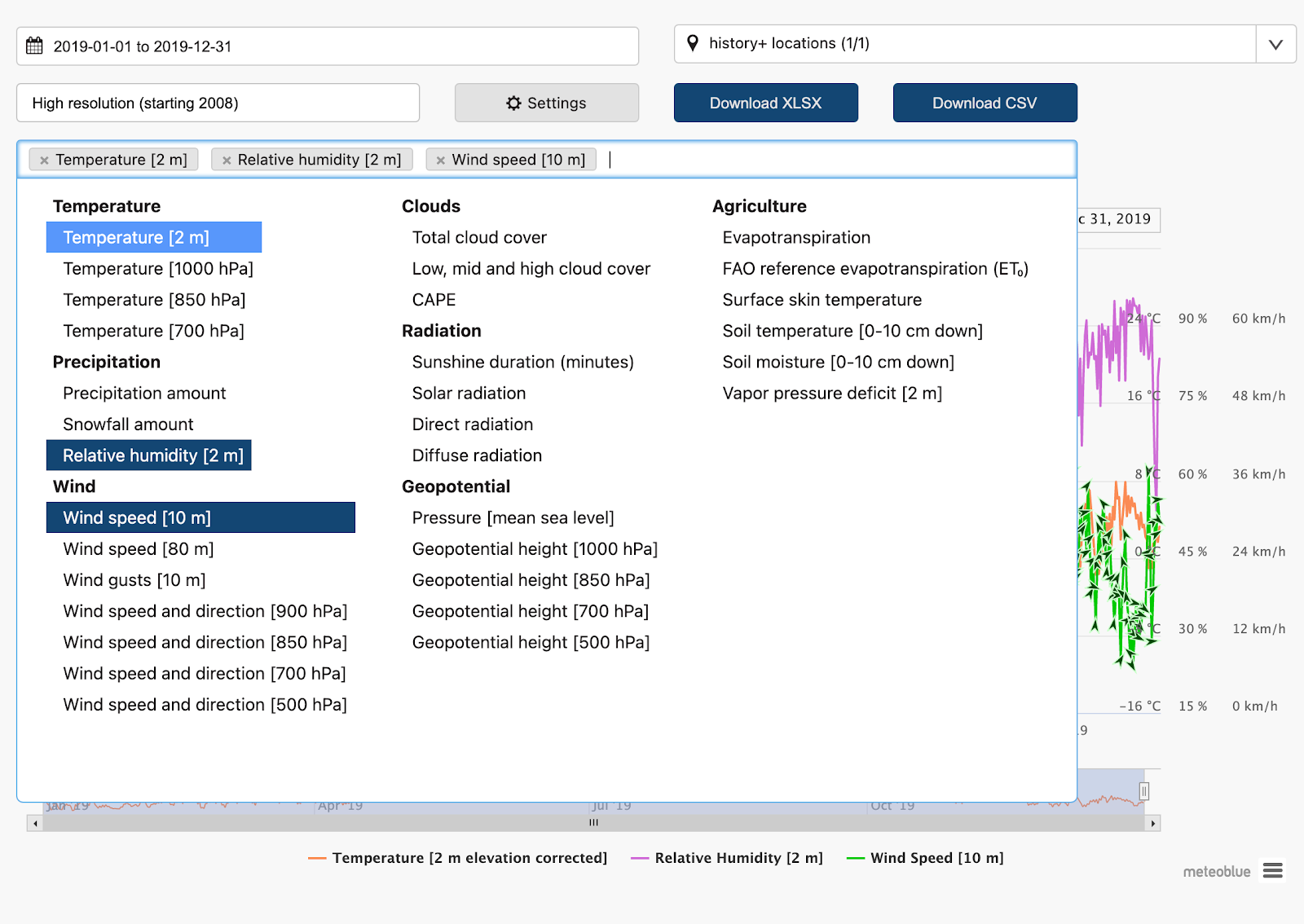
The data has been downloaded into a CSV file and requires minor processing.
Daylight
There is one other data source that I have used. Day length for every location on Earth changes during the year, with an average of 12 hours of light.
We should generate the length of each day of the year and the times of sunrises and sunsets. They will be needed later to resample the weather data.
from astral.sun import sun
from astral.sun import daylight
from astral import LocationInfo

class Helpers:
    @staticmethod
    def localtime_to_utc(date, local_timezone="Europe/Warsaw"):
        local = pytz.timezone(local_timezone)
        naive = datetime.datetime.strptime (date, "%Y-%m-%d %H:%M:%S")
        local_dt = local.localize(naive, is_dst=True)
        utc_dt = local_dt.astimezone(pytz.utc)
        return utc_dt.strftime ("%Y-%m-%d %H:%M:%S")

    @staticmethod
    def generate_daylight(start_date, end_date):
        datelist = pd.date_range(start_date, end=end_date).tolist()
        daylightData = pd.DataFrame(columns=['date','daylight','sunrise','sunset'])
        for date in datelist:
            daylight = Helpers.getDaylight(date)
            daylightData = daylightData.append({
                "date": date,
                "daylight": daylight['duration'],
                "sunrise": daylight['sunrise'],
                "sunset": daylight['sunset']
            }, ignore_index=True)
        return daylightData

    @staticmethod
    def getDaylight(start_date, timezone="Europe/Warsaw"):
        city = LocationInfo("Skitlawki", "Poland", timezone, LATITUDE, LONGITUDE)
        s = sun(city.observer, date=start_date)
        return {
            "duration": (s['sunset'] - s['sunrise']).seconds,
            "sunrise": s['sunrise'].strftime ("%Y-%m-%d %H:%M:%S"),
            "sunset": s['sunset'].strftime ("%Y-%m-%d %H:%M:%S")
        }
Collecting all data for the final set
Let’s gather all data (energy, weather and daylight) in one DataFrame.
dataset = pd.merge(left=meteoblue, right=daylight)
dataset['sunrise'] = pd.to_datetime(dataset['sunrise'])
dataset['sunset'] = pd.to_datetime(dataset['sunset'])
dataset['is_day'] = dataset[['ds','sunrise','sunset']].apply(lambda x: x['sunrise'] <= x['ds'] <= x['sunset'],  axis=1)
display(dataset.head())

df = dataset.loc[dataset['is_day']].drop('is_day', axis=1)

aggregations_dict = {
    'Temperature [2 m elevation corrected]': 'mean',
    'Temperature [1000 mb]': 'mean',
    'Temperature [850 mb]': 'mean',
    'Temperature [700 mb]': 'mean',
    'Precipitation Total': 'sum',
    'Snowfall Amount': 'sum',
    'Relative Humidity [2 m]': 'mean',
# (...)
    'Temperature': 'mean',
    'Soil Temperature [0-10 cm down]': 'mean',
    'Soil Moisture [0-10 cm down]': 'mean',
    'Vapor Pressure Deficit [2 m]': 'mean',
    'daylight': 'mean',
}


for key in aggregations_dict.keys():
    df[key] = pd.to_numeric(df[key])

df = df.resample('D', on='ds').agg(aggregations_dict).reset_index()
df = pd.merge(left=data.drop('ds', axis=1).drop(['cap','floor'], axis=1), right=df, left_on='ds', right_on='ds')
The resulting set has 46 columns, so a sample is shown here as raw CSV (full file: final_dataset_sample.csv):
ds,y,Temperature [2 m elevation corrected],Temperature [1000 mb],Temperature [850 mb],Temperature [700 mb],Precipitation Total,Snowfall Amount,Relative Humidity [2 m],Wind Speed [10 m],Wind Direction [10 m],Wind Speed [80 m],Wind Direction [80 m],Wind Gust,Wind Speed [900 mb],Wind Direction [900 mb],Wind Speed [850 mb],Wind Direction [850 mb],Wind Speed [700 mb],Wind Direction [700 mb],Wind Speed [500 mb],Wind Direction [500 mb],Cloud Cover Total,Cloud Cover High [high cld lay],Cloud Cover Medium [mid cld lay],Cloud Cover Low [low cld lay],CAPE [180-0 mb above gnd],Sunshine Duration,Shortwave Radiation,Direct Shortwave Radiation,Diffuse Shortwave Radiation,Mean Sea Level Pressure [MSL],Geopotential Height [1000 mb],Geopotential Height [850 mb],Geopotential Height [700 mb],Geopotential Height [500 mb],Evapotranspiration,FAO Reference Evapotranspiration [2 m],Temperature,Soil Temperature [0-10 cm down],Soil Moisture [0-10 cm down],Vapor Pressure Deficit [2 m],daylight,ds,cap,floor
2019-05-09,32425.0,12.64,12.65,2.47,-5.80,0.30,0.0,54.31,...,56060,2019-05-09,71061.0,0.0
2019-05-10,32269.0,13.85,13.60,2.99,-5.70,0.20,0.0,72.25,...,56276,2019-05-10,71061.0,0.0
Final dataset
Forecasting
To select external variables from a previously prepared dataset, we focus on two characteristics. First is the physical influence of variables, such as temperature and solar power reaching PV cells’ surface. Second is the correlation with the target variable. As we cannot be sure that some weather-related variable isn’t correlated somehow with another, which is directly tied with the effectiveness of solar farm, but unavailable to measure directly.
correlation_table = df.corr()
target_correlation_table = correlation_table.loc[correlation_table.index ** 'y'].transpose()

regressors = target_correlation_table.loc[np.abs(target_correlation_table['y']) >= 0.1].index.values
display(regressors)
The method of selecting variables was straightforward. First, we should reject variables with a close to zero correlation with the target variable. Let’s see how the model is doing with the remaining variables.
def prophet_with_regressors(train, test):
    m = Prophet(daily_seasonality=False, weekly_seasonality=False, yearly_seasonality=True, growth='logistic')
    for col in train.columns:
        if col in regressors and col not in ['y', 'cap', 'floor','Naive','Moving Average']:
            m.add_regressor(col)

    m.fit(train)

    forecast = m.predict(test)
    forecast['yhat'] = forecast['yhat'].apply(lambda x: 0 if x<0 else x)

    return forecast.rename(columns={'yhat':'y'}).set_index('ds')['y']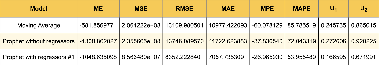
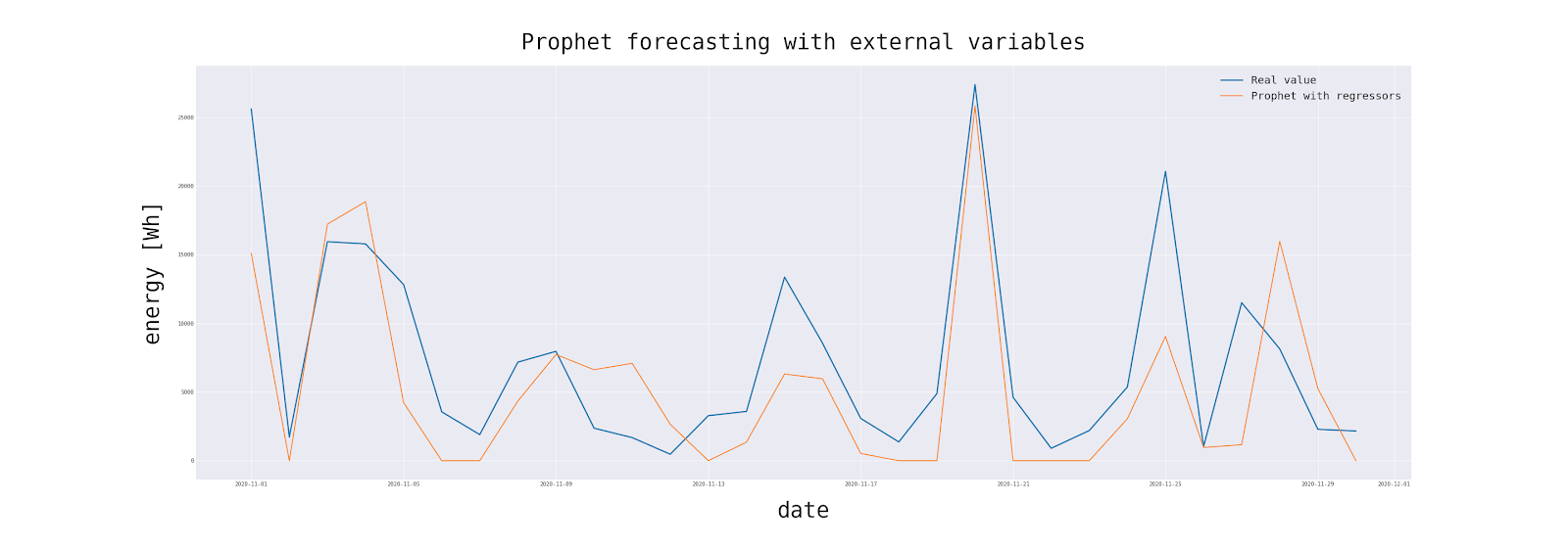
Quite a good one. Not only does the model have the best statistics so far, but it is also able to inform in advance about sudden changes in production values. The MSE is an order of magnitude smaller than previous attempts!
Limiting the number of necessary regressors
Variables such as Shortwave Radiation are obviously linked to solar electricity production, but at the same time are not easily accessible in the weather forecast. Therefore, we will now try to limit the number of variables to the necessary minimum and to those that can be found in any weather forecast.
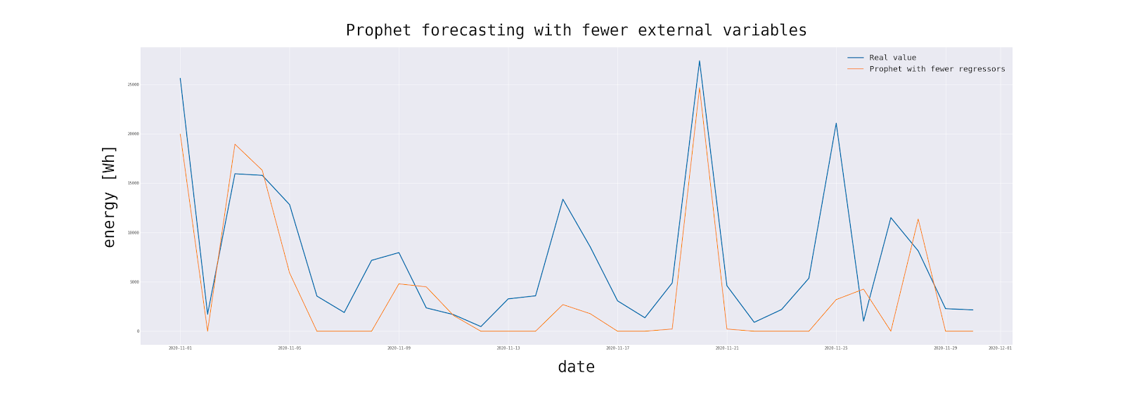
Quite close to the ‘full’ model.
Conclusions
With the use of a relatively small number of weather variables, electricity production by PV cells can be predicted with satisfactory accuracy. Importantly, the predictions of explanatory variables are easily accessible in most weather forecasts. However, if we use all measurable variables, the model achieves correspondingly better results.
Future directions
Predictive models, aware of how prices, supply and demand are shaped and knowing future forecasts of energy production, can prepare recommendations for owners as to their behaviour on the energy market. This can create additional revenue opportunities for users of renewable energy sources.
My friends have a smart home solution. They already integrate their lights in it and schedule dishwasher or washing machine cycles with potential high PV activity. In the future, all of their power plugs could be scheduled by solar prediction. Another direction is to provide the forecasts in the form of a kitchen dashboard.
References
- https://www.solaredge.com/sites/default/files/se_monitoring_api.pdf
- http://www.geo.mtu.edu/KeweenawGeoheritage/MiTEP_ESI-2/Solar_energy_and_latitude.html
- https://otexts.com/fpp2/accuracy.html
- https://www.thegreenage.co.uk/article/the-impact-of-temperature-on-solar-panels/