Measuring forecast accuracy
Forecast evaluation statistics with examples in Python
If I had to choose one basic skill in data science that is the most useful, it would be time series forecasting. Predicting the future value of something contributes to making better decisions. Therefore, it is crucial to be sure that you can rely on forecasting. The choosing, construction and interpretation of forecast accuracy metrics are just as important as making forecasts.
What actually makes up the accuracy of the forecast?

How to choose evaluation statistics
Choosing a accuracy estimation method often depends on the domain of the problem. In my career, I have encountered a situation where a hastily chosen metric has caused the client’s dissatisfaction with the forecasting results optimized for KPI inconsistent with the specific business case. For example, the model may have a low mean square error, but at the same time doesn’t predict sudden deviations from “everyday normal” values or trend changes.
This article will show you the fundamental forecast evaluation statistics that you can use to build and test your predictive models. We will calculate and interpret them using concrete examples: the mean error (ME), the mean squared error (MSE), the mean absolute error (MAE), the mean percentage error (MPE), the mean absolute percentage error (MAPE), and Theil’s U-statistics. We will interpret and discuss examples in Python in the context of time-series forecasting data.
Note: As I am focusing on specific metrics in this article, I do not address the subject of cross-validation and the splitting of the data set into training and testing. As this is an important concept, I plan to address this topic in future texts.
Why?
Imagine that you work for an electricity producer. Your task is to create a model that predicts the daily production of electricity in a small wind farm. This will make it possible to plan and reduce the production of electricity in a conventional power station at times of high efficiency from renewable sources.

You have created a couple of prediction models. How to choose the best one to do the task?
Dataset
To allow the calculation of all presented statistics, a CSV file has been created.
| ds | y | Naive | Moving Average | Advanced #1 | Advanced #2 |
|---|---|---|---|---|---|
| 2020-04-01 | 11534.0 | 10579.0 | 13435.0 | ||
| 2020-04-02 | 16063.0 | 11534.0 | 23928.0 | 18007.0 | |
| 2020-04-03 | 34138.0 | 16063.0 | 34263.0 | 27723.0 | |
| 2020-04-04 | 34091.0 | 34138.0 | 41914.0 | 35713.0 | |
| 2020-04-05 | 58414.0 | 34091.0 | 23956.0 | 47230.0 | 53892.0 |
| 2020-04-06 | 61080.0 | 58414.0 | 35676.0 | 50566.0 | 59580.0 |
| 2020-04-07 | 56992.0 | 61080.0 | 46931.0 | 52275.0 | 59721.0 |
| 2020-04-08 | 61045.0 | 56992.0 | 52644.0 | 52697.0 | 61959.0 |
| 2020-04-09 | 36327.0 | 61045.0 | 59383.0 | 52151.0 | 47474.0 |
| 2020-04-10 | 54514.0 | 36327.0 | 53861.0 | 50929.0 | 53416.0 |
First 10 rows of 91. Full data: fes.csv
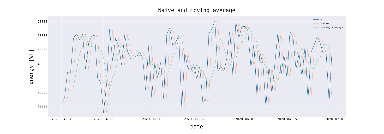
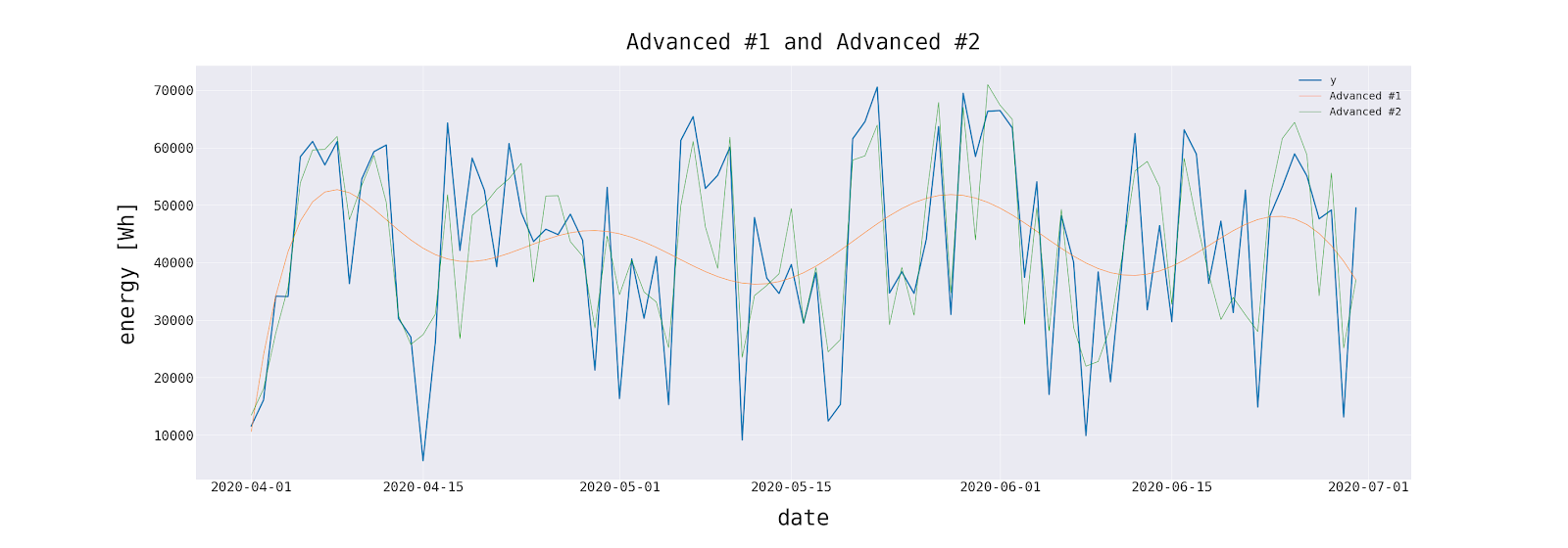
This spreadsheet contains an example involving two months of observations and four alternative sets of forecasts (made with naive, moving average and two more advanced methods) of a variable of interest (denoted as y).
Technical details
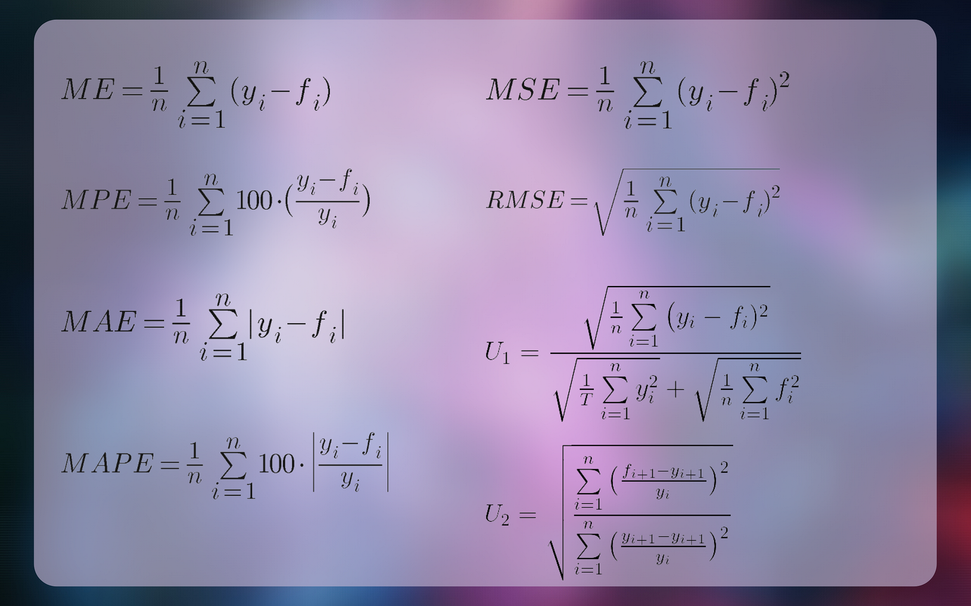
The notation used below is fairly standard, with yᵢ and fᵢ as a variable of interest and forecast respectively, and n as a number of observations. Full source code used for preparing this article:
To avoid repetition in the code, I sketched a simple class FES, with static methods that calculate each statistic. This makes the code more readable, without the risk of functions’ name conflict.
Forecast evaluation statistics
By an “error” we mean uncertainty in forecasting, or, in other words, the difference between the predicted value and real value. It is a yᵢ — fᵢ component in most of the following formulas.
Mean error
The mean error is the average of all the errors in a set.
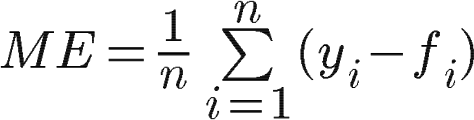
This is a very simple statistic. Unfortunately is biased due to the offsetting effect of positive and negative forecast errors, which may conceal forecasting inaccuracy. Because of that, ME isn’t very helpful to model evaluation. However, it is very easy to understand, even for a layman (this is not always an advantage, because of the limitations described above). ME can quickly present the symmetry of the error distribution, which can be useful in assessing a specific model.
def me(f,y):
    f = f.reset_index(drop=True).values.flatten()
    y = y.reset_index(drop=True).values.flatten()
    df = pd.DataFrame({'f_i':f, 'y_i': y})
    df['e'] = df['y_i'] - df['f_i']
    return np.mean(df['e'])
Mean absolute error
A remedy for the inaccuracy of the mean error is the use of the mean absolute error.
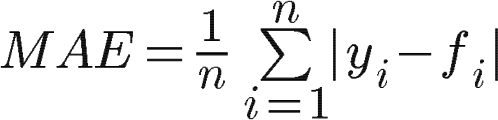
The MAE uses absolute values of errors in the calculations, which overcomes the cancellation of errors with opposite signs. It gives us an average of all values of errors, no matter whether they were positive or negative.
def mae(f, y):
    f = f.reset_index(drop=True).values.flatten()
    y = y.reset_index(drop=True).values.flatten()
    df = pd.DataFrame({'f_i':f, 'y_i': y})
    df['e'] = np.abs(df['y_i'] - df['f_i'])
    return np.mean(df['e'])
Mean square error
Just like the MAE, mean square error overcomes the cancellation of positive and negative errors.
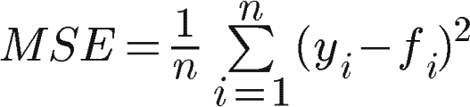
Also, the MSE places a greater penalty on large forecast errors than the MAE.
def mse(f, y):
    f = f.reset_index(drop=True).values.flatten()
    y = y.reset_index(drop=True).values.flatten()
    df = pd.DataFrame({'f_i':f, 'y_i': y})
    df['e'] = np.square(df['y_i'] - df['f_i'])
    return np.mean(df['e'])
Root mean square error
Root mean square error is the standard deviation of the errors.
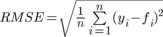
RMSE shares advantages of MSE and is commonly used in forecasting and regression analysis to verify experimental results. Furthermore, it has the advantage of having the same units as the forecasted variable, so it is easier to directly interpret.
def rmse(f, y):
    return np.sqrt(mse(f,y))
Mean percentage error
Mean percentage error is the average of percentage errors by which each forecast differs from corresponding real observed values.
This statistic is easy to understand because it provides the error in terms of percentages. As in the ME, positive and negative forecast errors can offset each other, so it can be used to measure bias in the forecasts. The disadvantage of this statistic is that it is not suitable for datasets containing observed values, which are equal to zero.
def mpe(f, y):
    f = f.reset_index(drop=True).values.flatten()
    y = y.reset_index(drop=True).values.flatten()
    df = pd.DataFrame({'f_i':f, 'y_i': y})
    df['e'] = df['y_i'] - df['f_i']
    df['pe'] = 100*(df['e']/df['y_i'])
    return np.mean(df['pe'])
Mean absolute percentage error
The mean absolute percentage error overcomes the problem with error offsetting and works best if there are no extremes to the data (and no zeros).
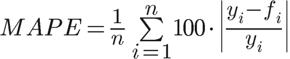
def mape(f, y):
    f = f.reset_index(drop=True).values.flatten()
    y = y.reset_index(drop=True).values.flatten()
    df = pd.DataFrame({'f_i':f, 'y_i': y})
    df['e'] = df['y_i'] - df['f_i']
    df['ape'] = 100*np.abs(df['e']/df['y_i'])
    return np.mean(df['ape'])
Theil’s U statistics
There is some confusion about Theil’s forecast accuracy coefficient, caused probably by Theil himself. He proposed two different formulas at different times under the same name, both labelled with U. More about this topic you find in Forecast Evaluation using Theil’s Inequality Coefficients.
U₁
The values of U₁ are in the range (0, 1).

The greater accuracy of the forecast, the lower will be the value of the U₁.
def u1(f,y):
    y = y.reset_index(drop=True).values.flatten()
    f = f.reset_index(drop=True).values.flatten()
    df = pd.DataFrame({'f_i':f, 'y_i': y})
    df['(f_i - y_i)^2'] = np.square(df['f_i'] - df['y_i'])
    df['y_i^2'] = np.square(df['y_i'])
    df['f_i^2'] = np.square(df['f_i'])
    return (np.sqrt(np.mean(df['(f_i - y_i)^2'])))/(np.sqrt(np.mean(df['y_i^2']))+np.sqrt(np.mean(df['f_i^2'])))
U₂
Theil’s U₂ tells how much more (or less) accurate a model is relative to a naïve forecast.

U₂ has a lower bound of 0 (which indicates perfect forecast), hasn’t an upper limit. When the value of U₂ thing exceeds 1, it means that the forecast method becomes doing worse than naive forecasting.
def u2(f,y):
    y = y.reset_index(drop=True).values.flatten()
    f = f.reset_index(drop=True).values.flatten()
    df = pd.DataFrame({'f_i+1':f, 'y_i+1': y})
    df['y_i'] = df['y_i+1'].shift(periods=1)
    df['numerator'] = np.square((df['f_i+1'] - df['y_i+1']) / df['y_i'])
    df['denominator'] = np.square((df['y_i+1'] - df['y_i']) / df['y_i'])
    df.dropna(inplace=True)
    return np.sqrt(np.sum(df['numerator'])/np.sum(df['denominator']))
Model evaluation
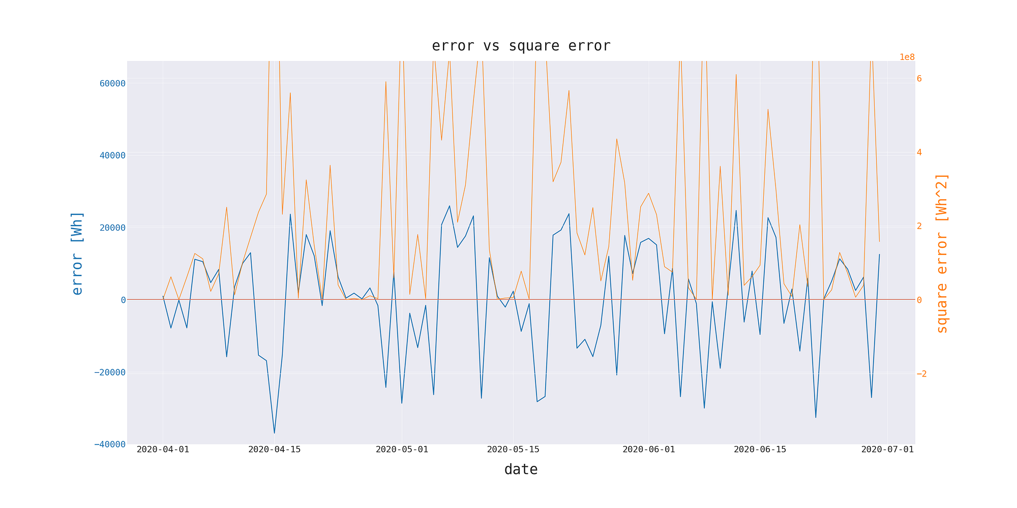
Let’s go back to our dataset. It contains the results of 4 different predictive models.
The table below contains all the statistics described in this article, calculated for each model.
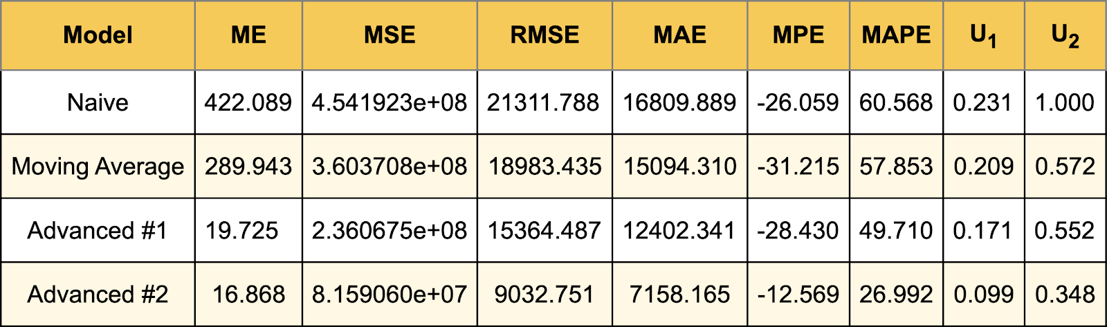
It is worth noting that the advanced method has a square error of an order of magnitude smaller than any other. It is also a top performer in other statistics.
Conclusions
If the main indicator of success was the ability of the model to inform about sudden changes in the predicted variable, then “Advanced #2” will be the preferred method. This is consistent with the intuition and visual evaluation of the plot. However, this method is the most complex in terms of calculation and requires the use of external variables. But in such an important domain of the problem as electricity generation, this is an acceptable cost.
The “Advanced #1” and moving averages methods, on the other hand, are suitable for rough estimates. The above conclusions would be impossible to draw without looking at alternative statistics, which shows that no forecast evaluation statistic is redundant as each has information to impart.
I used the described statistics in practice when creating models:
How to predict solar energy production — Efficient use of renewable energy sources with machine learning
How to Forecast Website Traffic — Local Pageview Projection Tool using Weather Data
References
- http://www.treasury.act.gov.au/documents/Forecasting%20Accuracy%20-%20ACT%20Budget.pdf
- https://www.economicsnetwork.ac.uk/showcase/cook_forecast
- https://www.jstor.org/stable/2352722?seq=1
- https://stackoverflow.com/questions/54931514/theils-u-1-theils-u-2-forecast-coefficient-formula-in-python
- https://stats.stackexchange.com/questions/345178/interpretation-of-theils-u2-statistic-forecasting-methods-and-applications
- https://docs.oracle.com/cd/E40248_01/epm.1112/cb_statistical/frameset.htm?ch07s02s03s04.html
- https://www.statisticshowto.com/mean-error/
- https://en.wikipedia.org/wiki/Mean_percentage_error
- https://arxiv.org/abs/1905.11744